A look at GDP of US,India & Germany across the years
GDP components over time and among countries
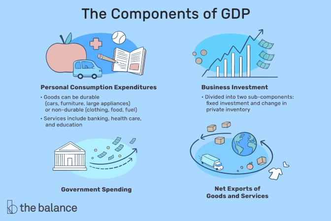
At the risk of oversimplifying things, the main components of gross domestic product, GDP are personal consumption (C), business investment (I), government spending (G) and net exports (exports - imports). You can read more about GDP and the different approaches in calculating at the Wikipedia GDP page.
The GDP data we will look at is from the United Nations’ National Accounts Main Aggregates Database, which contains estimates of total GDP and its components for all countries from 1970 to today. We will look at how GDP and its components have changed over time, and compare different countries and how much each component contributes to that country’s GDP. The file we will work with is GDP and its breakdown at constant 2010 prices in US Dollars and it has already been saved in the Data directory. Have a look at the Excel file to see how it is structured and organised
Reading the GDP Data
UN_GDP_data  <-  read_excel(here::here("data", "Download-GDPconstant-USD-countries.xls"), # Excel filename
                sheet="Download-GDPconstant-USD-countr", # Sheet name
                skip=2) # Number of rows to skip
Tidying the data
# Tidy GDP data by 1) pivoting it long, 2) mutate GDP to in billions
tidy_GDP_data <- UN_GDP_data %>%
  pivot_longer(cols = 4:51,
               values_to = "GDP",
               names_to = "Year") %>%
  mutate(GDP = GDP/1e9)

glimpse(tidy_GDP_data)
## Rows: 176,880
## Columns: 5
## $ CountryID <dbl> 4, 4, 4, 4, 4, 4, 4, 4, 4, 4, 4, 4, 4, 4, 4, 4, 4, 4, 4,…
## $ Country <chr> "Afghanistan", "Afghanistan", "Afghanistan", "Afghanista…
## $ IndicatorName <chr> "Final consumption expenditure", "Final consumption expe…
## $ Year <chr> "1970", "1971", "1972", "1973", "1974", "1975", "1976", …
## $ GDP <dbl> 5.56, 5.33, 5.20, 5.75, 6.15, 6.32, 6.37, 6.90, 7.09, 6.…# Let us compare GDP components for these 3 countries
country_list <- c("United States","India", "Germany")
# Select GDP for these three countries only
US_India_Germany <- tidy_GDP_data %>%
filter(Country %in% country_list)
glimpse(US_India_Germany)## Rows: 2,448
## Columns: 5
## $ CountryID <dbl> 276, 276, 276, 276, 276, 276, 276, 276, 276, 276, 276, 2…
## $ Country <chr> "Germany", "Germany", "Germany", "Germany", "Germany", "…
## $ IndicatorName <chr> "Final consumption expenditure", "Final consumption expe…
## $ Year <chr> "1970", "1971", "1972", "1973", "1974", "1975", "1976", …
## $ GDP <dbl> 1152, 1218, 1282, 1329, 1345, 1398, 1450, 1504, 1560, 16…GDP Breakdown & its variations
indicator_of_interest <- c("Gross capital formation", "Exports of goods and services", "General government final consumption expenditure", "Household consumption expenditure (including Non-profit institutions serving households)", "Imports of goods and services")

selected_US_India_Germany <- US_India_Germany %>%
  filter(IndicatorName %in% indicator_of_interest) %>%
  mutate(Year = as.numeric(Year), IndicatorName = factor(IndicatorName, levels = c("Gross capital formation", "Exports of goods and services", "General government final consumption expenditure", "Household consumption expenditure (including Non-profit institutions serving households)", "Imports of goods and services"),labels = c("Gross capital formation","Exports","Government Expenditure","Household Expenditure","Imports")))

ggplot(data = selected_US_India_Germany, aes(x = Year, y = GDP, colour = IndicatorName)) +
  geom_line() +
  labs(title="GDP Components over time", subtitle="In constant 2010 USD",y="Billion US$") +
  facet_wrap(~ Country) +
  theme_bw() +
  #theme(legend.title = "Components of GDP") +
  NULL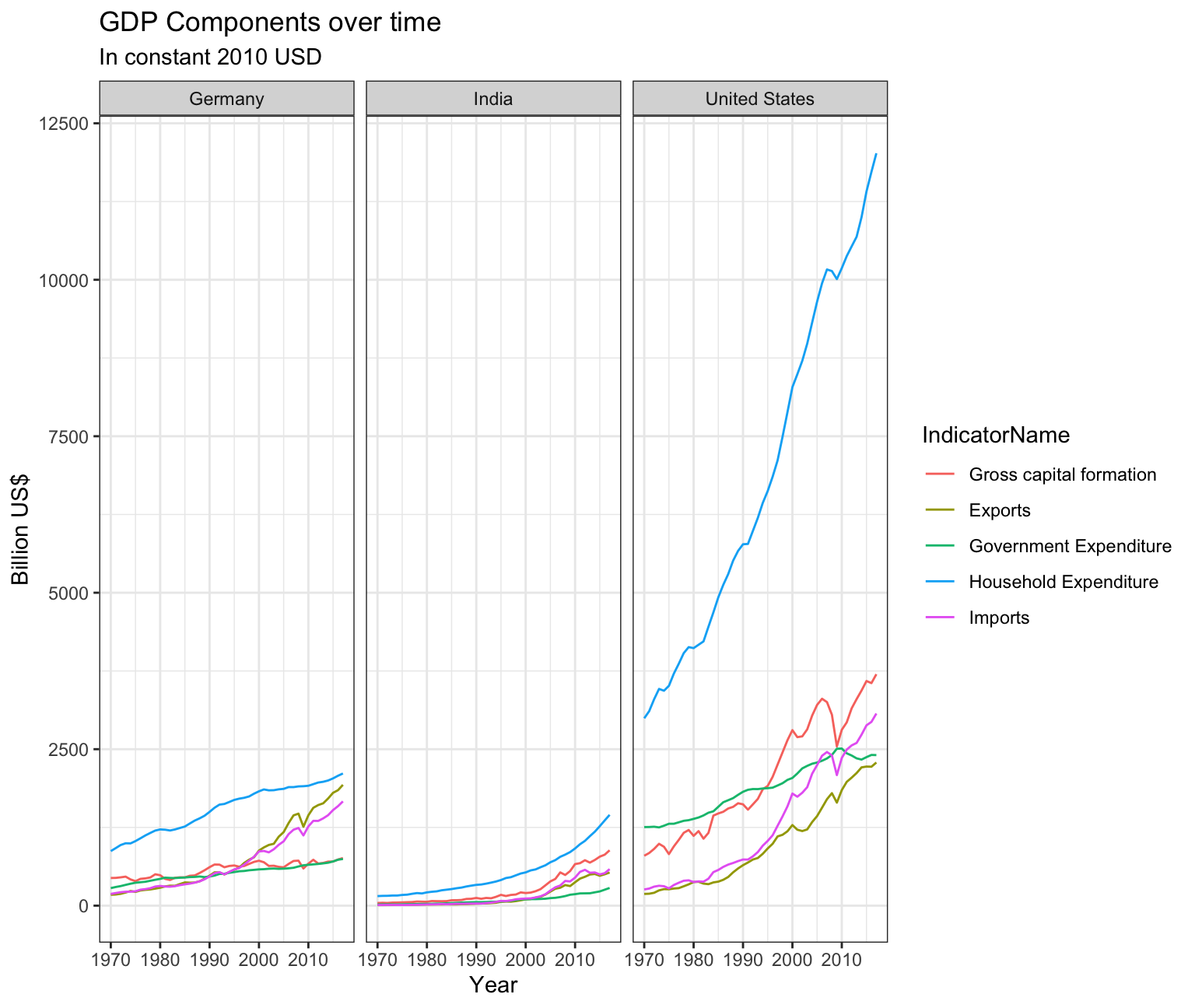
Secondly, recall that GDP is the sum of Household Expenditure (Consumption C), Gross Capital Formation (business investment I), Government Expenditure (G) and Net Exports (exports - imports). Even though there is an indicator Gross Domestic Product (GDP) in your dataframe, I would like you to calculate it given its components discussed above.
new_indicator_of_interest <- c("Gross capital formation", "Exports of goods and services", "General government final consumption expenditure", "Household consumption expenditure (including Non-profit institutions serving households)", "Imports of goods and services", "Gross Domestic Product (GDP)")

new_selected_US_India_Germany <- US_India_Germany %>%
  filter(IndicatorName %in% new_indicator_of_interest) %>%
  mutate(Year = as.numeric(Year))

reorder <- c("country_id", "country", "year", "gross_domestic_product_gdp","GDP_calc", "household_consumption_expenditure_including_non_profit_institutions_serving_households", "general_government_final_consumption_expenditure", "gross_capital_formation", "net_exports")


wide_new_selected_US_India_Germany <- new_selected_US_India_Germany %>%
  pivot_wider(names_from = IndicatorName, values_from = GDP) %>%
  janitor::clean_names() %>%
  mutate(net_exports = exports_of_goods_and_services - imports_of_goods_and_services,GDP_calc=(household_consumption_expenditure_including_non_profit_institutions_serving_households+general_government_final_consumption_expenditure+gross_capital_formation+net_exports)) %>%
  select(-c(exports_of_goods_and_services, imports_of_goods_and_services)) %>%
  select(reorder)

long_new_selected_US_India_Germany <- wide_new_selected_US_India_Germany %>%
  pivot_longer(cols = c(6:9),
             names_to = "component",
             values_to = "value") %>%
  mutate(percentage = value/GDP_calc,component=factor(component,levels=c("general_government_final_consumption_expenditure","gross_capital_formation","household_consumption_expenditure_including_non_profit_institutions_serving_households","net_exports"),labels=c("Government Expenditure","Gross Capital Formation","Household Expenditure","Net Exports")))

long_new_selected_US_India_Germany <- long_new_selected_US_India_Germany %>%
  mutate(GDP_change=100*(GDP_calc-gross_domestic_product_gdp)/GDP_calc )

ggplot(data = long_new_selected_US_India_Germany, aes(x = year, y = percentage, colour = component)) +
  geom_line() +
  labs(title="GDP and its breakdown at constant 2010 prices in US Dollars",x="",y="Proportion",caption="Source: United Nations, https://unstats.un.orq/unsd/snaama/Downloads") +
  facet_wrap(~country) +
  theme_bw() +
  theme(legend.title = element_blank()) +
  NULL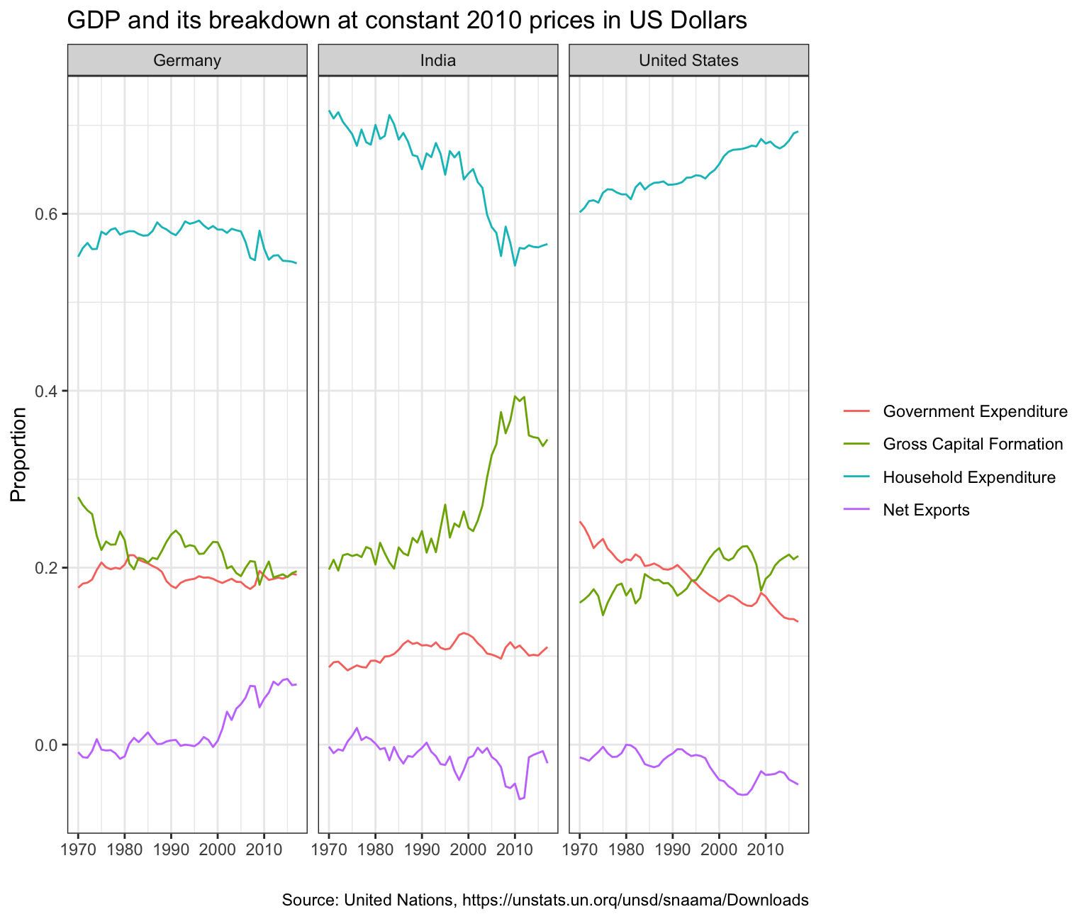
The Gross Capital Formation and Government Expenditure has switched places multiple times although the Gross Capital Formation has historically kept a higher proportion of GDP. After 2010, these two have kept a pretty even share at ~20% each. The Net exports have improved post the 2000.
The GDP contribution of Household Expenditure of India has been on a consistent downtrend from the 1980’s(70%-55%) whereas the Gross capital formation contribution has improved and spiked after the 2000’s. Net Exports and Governemtn Expenditure has remained pretty stable over the years, other than the dips in the Net Exports during the late 1990’s and the late 2000’s.
For The United States, the contribution for all 4 components have remained relatively stable. Only noticeable change is the Gross Capital Formation component(Increasing trend) increasing to go above the Government Expenditure component(Descending trend) in the 1990’s. The Household Expenditure has a slow but stable increase over the years while the Net Exports have decreased marginally, although with dips in between.
#Difference in calculated & given GDP
ggplot(long_new_selected_US_India_Germany, aes(x=year,y=GDP_change)) +
  geom_line() +
  facet_wrap(~country)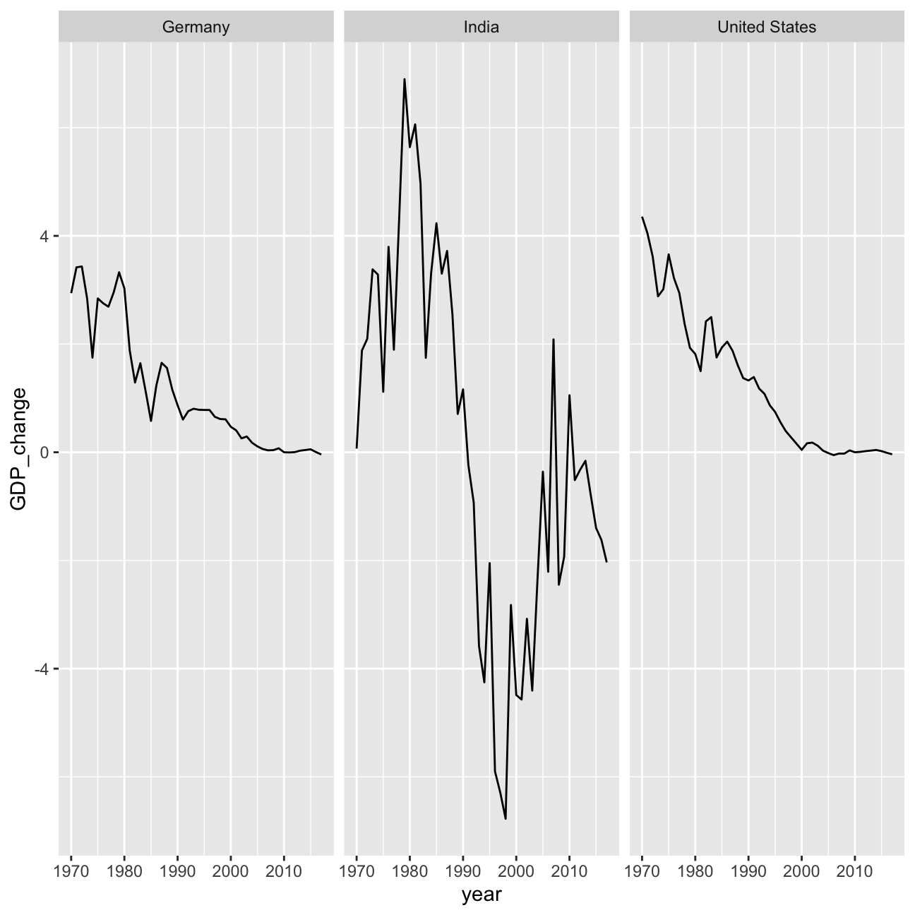
According to the graph created, the % of difference between GDP calculated and Given GDP varies a lot for India. The same for Germany & United States used to be very variable, but post 2000’s, the differences are negligible.